Fetch Tutorial¶

The python module cheta.fetch provides a simple interface to the engineering archive data files. Using the module functions it is easy to retrieve data over a time range for a single MSID or a related set of MSIDs. The data are return as MSID objects that contain not only the telemetry timestamps and values but also various other data arrays and MSID metadata.

Getting started¶

First fetch

The basic process of fetching data always starts with importing the module into the python session:

import cheta.fetch as fetch

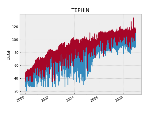
The as fetch part of the import statement just creates an short alias to avoid always typing the somewhat lengthy cheta.fetch.MSID(..). Fetching and plotting full time-resolution data for a single MSID is then quite easy:

tephin = fetch.MSID('tephin', '2009:001', '2009:007') # (MSID, start, stop)
clf()
plot(tephin.times, tephin.vals)

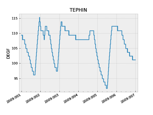
The tephin variable returned by MSID() is an MSID object and we can access the various object attributes with <object>.<attr>. The timestamps tephin.times and the telemetry values tephin.vals are both numpy arrays. As such you can inspect them and perform numpy operations and explore their methods:

type(tephin)
type(tephin.vals)
help tephin.vals
tephin.vals.mean()
tephin.vals.min()
tephin.vals.<TAB>
tephin.times[1:20]
tephin.vals[1:20]

Default start and stop values

If you do not provide a value for the start time, then it defaults to the beginning of the mission (1999:204 = July 23, 1999). If you do not provide a stop time then it defaults to the latest available data in the archive.

tephin = fetch.Msid('tephin', stop='2001:001') # Launch through 2001:001
tephin = fetch.Msid('tephin', start='2010:001') # 2010:001 through NOW
tephin = fetch.Msid('tephin', '2010:001') # Same as previous
tephin = fetch.Msid('tephin') # Launch through NOW

Derived parameters (calcs)

The engineering archive has pseudo-MSIDs that are derived via calculation from telemetry MSIDs. These are also known as “calcs” in the context of MAUDE. In MAUDE, a calc is normally indicated with a prefix of CALC_, but for compatibility with cheta a prefix of DP_ is also allowed.

Derived parameter names begin with the characters DP_ (not case sensitive as usual). Otherwise there is no difference from standard MSIDs. When querying the archive using fetch, there are three equivalent ways to specify an MSID name:

DP_<name>> e.g. DP_PITCH_FSS
CALC_<name> e.g. CALC_PITCH_FSS
<name> e.g. PITCH_FSS: this is a convenience and internally fetch will search for derived parameters matching DP_<name>.

See the Derived Parameters or Calcs section for more details and full listings of available MSIDs.

Other details

If you are wondering what time range of data is available for a particular MSID use the get_time_range() function:

fetch.get_time_range('tephin', format='date')
('1999:365:22:40:33.076', '2013:276:12:04:39.361')

The name of the variable holding the MSID object is independent of the MSID name itself. Case is not important when specifying the MSID name so one might do:

pcad_mode = fetch.MSID('AOpcadMD', '2009Jan01 at 12:00:00.000', '2009-01-12T14:15:16')
pcad_mode.msid  # MSID name as entered by user
pcad_mode.MSID  # Upper-cased version used internally

The times attribute gives the timestamps in elapsed seconds since 1998-01-01T00:00:00. This is the start of 1998 in Terrestrial Time (TT) and forms the basis for time for all CXC data files. In order to make life inconvenient 1998-01-01T00:00:00 is actually 1997:365:23:58:56.816 (UTC). This stems from the difference of around 64 seconds between TT and UTC.

Date and time formats¶

The Ska engineering telemetry archive tools support a wide range of formats for representing date-time stamps. Note that within this and other documents for this tool suite, the words ‘time’ and ‘date’ are used interchangably to mean a date-time stamp.

The available formats are listed in the table below:

Format	Description	System
secs	Elapsed seconds since 1998-01-01T00:00:00	tt
numday	DDDD:hh:mm:ss.ss… Elapsed days and time	utc
jd*	Julian Day	utc
mjd*	Modified Julian Day = JD - 2400000.5	utc
date	YYYY:DDD:hh:mm:ss.ss..	utc
caldate	YYYYMonDD at hh:mm:ss.ss..	utc
fits	FITS date/time format YYYY-MM-DDThh:mm:ss.ss..	tt
unix*	Unix time (since 1970.0)	utc
greta	YYYYDDD.hhmmss[sss]	utc

* Ambiguous for input parsing and only available as output formats.

For the date format one can supply only YYYY:DDD in which case 12:00:00.000 is implied.

The default time “System” for the different formats is either tt (Terrestrial Time) or utc (UTC). Since TT differs from UTC by around 64 seconds it is important to be consistent in specifying the time format.

Converting between units is straightforward with the Chandra.Time module:

import Chandra.Time
datetime = Chandra.Time.DateTime(126446464.184)
datetime.date
Out[]: '2002:003:12:00:00.000'

datetime.greta
Out[]: '2002003.120000000'

Chandra.Time.DateTime('2009:235:12:13:14').secs
Out[]: 367416860.18399996

Exporting to CSV¶

If you want to move the fetch data to your local machine an MSID or MSIDset can be exported as ASCII data table(s) in CSV format. This can easily be imported into Excel or other PC applications.:

biases = fetch.MSIDset(['aogbias1', 'aogbias2', 'aogbias3'], '2002:001', stat='daily')
biases.write_zip('biases.zip')

To suspend the ipython shell and look at the newly created file do:

<Ctrl>-z

% ls -l biases.zip
-rw-rw-r-- 1 aldcroft aldcroft 366924 Dec  4 17:07 biases.zip

% unzip -l biases.zip
Archive:  biases.zip
  Length     Date   Time    Name
 --------    ----   ----    ----
   510809  12-04-09 17:02   aogbias1.csv
   504556  12-04-09 17:02   aogbias2.csv
   504610  12-04-09 17:02   aogbias3.csv
 --------                   -------
  1519975                   3 files

To resume your ipython session:

% fg

From a separate local cygwin or terminal window then retrieve the zip file and unzip as follows:

scp ccosmos.cfa.harvard.edu:biases.zip ./
unzip biases.zip

Plotting time data¶

Even though seconds since 1998.0 is convenient for computations it isn’t so natural for humans. As mentioned the Chandra.Time module can help with converting between formats but for making plots we use the plot_cxctime() function of the Ska.Matplotlib module:

from Ska.Matplotlib import plot_cxctime
clf()
plot_cxctime(tephin.times, tephin.vals)

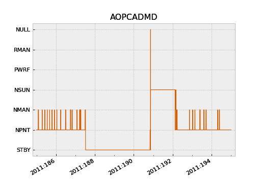
An even simpler way to make the same plot is with the plot() function:

tephin.plot()

That looks better:

Tip

The plot() method accepts any arguments work with the Matplotlib plot_date() function

Interactive plotting¶

The iplot() function is a handy way to quickly explore MSID data over a wide range of time scales, from seconds to the entire mission in a few key presses. The function automatically fetches data from the archive as needed.

When called this method opens a new plot figure (or clears the current figure) and plots the MSID vals versus times. This plot can be panned or zoomed arbitrarily and the data values will be fetched from the archive as needed. Depending on the time scale, iplot will display either full resolution, 5-minute, or daily values. For 5-minute and daily values the min and max values are also plotted.

Once the plot is displayed and the window is selected by clicking in it, the plot limits can be controlled by the usual methods (window selection, pan / zoom). In addition following key commands are recognized:

a: autoscale for full data range in x and y
m: toggle plotting of min/max values
p: pan at cursor x
y: toggle autoscaling of y-axis
z: zoom at cursor x
?: print help

Example:

dat = fetch.Msid('aoattqt1', '2011:001', '2012:001', stat='5min')
dat.iplot()

The iplot() and plot() functions support plotting state-valued MSIDs such as AOPCADMD or AOUNLOAD:

dat = fetch.Msid('aopcadmd', '2011:185', '2011:195')
dat.iplot()
grid()

Note

The iplot() method is not meant for use within scripts, and may give unexpected results if used in combination with other plotting commands directed at the same plot figure. Instead one should use the MSID plot() method in this case.

Data filtering¶

Often one needs to filter or select subsets of the raw telemetry that gets fetched from the archive in order to use the values in analysis. Here we describe the ways to accomplish this in different circumstances.

Event interval filtering¶

The first case is when one needs to either select or remove specific intervals of telemetry values from a full MSID() or MSIDset() object based on known spacecraft events. For instance when analyzing OBC rate noise we need to use only data during periods of stable Kalman lock. Likewise it is frequently useful to exclude time intervals during which the spacecraft was in an anomalous state and OBC telemetry is unreliable.

Using Kadi¶

Frequently one can handle this with the remove_intervals() select_intervals() methods in conjunction with the kadi event intervals mechanism.

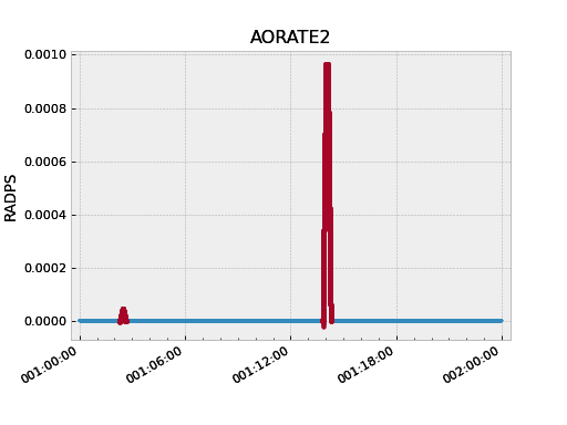
As a simple example, the following code fetches the pitch component of the spacecraft rate. The samples during maneuvers are then selected and then replotted. This highlights the large rates during maneuvers:

>>> aorate2 = fetch.Msid('aorate2', '2011:001', '2011:002')
>>> aorate2.iplot()

>>> from kadi import events
>>> aorate2.select_intervals(events.manvrs)
>>> aorate2.plot('.r')

(Source code, png, hires.png, pdf)

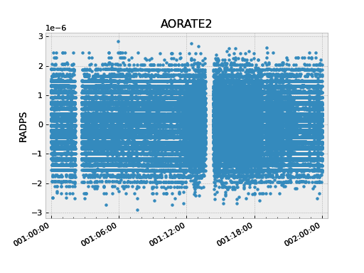
The following code illustrates use of the remove_intervals() method to select all all time intervals when the spacecraft is not maneuvering. In this case we include a pad time of 600 seconds before the start of a maneuver and 300 seconds after the end of each maneuver.

>>> aorate2 = fetch.Msid('aorate2', '2011:001', '2011:002')
>>> events.manvrs.interval_pad = (600, 300)  # Pad before, after each maneuver (seconds)
>>> aorate2.remove_intervals(events.manvrs)
>>> aorate2.iplot('.')

(Source code, png, hires.png, pdf)

Using logical intervals¶

For cases where the intervals to be filtered cannot be expressed as Kadi events, the approach is to use the logical_intervals() function located in the cheta.utils module. This function creates an intervals table where each row represents a desired interval and includes a datestart and datestop column.

For example to extract solar array temperatures when the off-nominal roll angle is between 5 and 10 degrees you would do:

>>> from cheta.utils import logical_intervals

>>> sa_temps = fetch.Msid('TSAPYT','2010:001',stat='5min')
>>> roll = fetch.Msid('ROLL','2010:001',stat='5min')

>>> roll_off_nom = (roll.vals > 5) & (roll.vals < 10)
>>> off_nom_intervals = logical_intervals(roll.times, roll_off_nom)

>>> sa_temps_off_nom = sa_temps.select_intervals(off_nom_intervals, copy=True)

>>> sa_temps.plot('.r')
>>> sa_temps_off_nom.plot('.b')

(Source code, png, hires.png, pdf)

Notice that we created a new version of the solar array temperatures MSID object called sa_temps_off_nom (using copy=True) instead of filtering in place. Sometimes it is convenient to have both the original and filtered data, e.g. when you want to plot both.

Note also that remove_intervals() select_intervals() will accept any table with columns datestart / datestop or tstart / tstop as input.

Fetching only small intervals¶

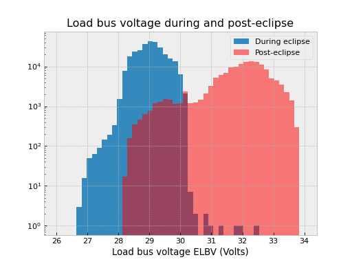
It may be the case that you want to fetch a number of small intervals of an MSID that is sampled at a high rate. An example is looking at the load bus voltage ELBV for 5 minutes after each eclipse. Because ELBV comes down in telemetry about 4 times per second, fetching all the values for the mission and then selecting intervals is prohibitively expensive in memory and time.

There is a different mechanism that can work in these situations. The start argument to a fetch.MSID or fetch.MSIDset query can be an interval specifier. This might be the output of logical_intervals() or it might just be a list of (start, stop) tuples. If that is the case then fetch will iterate through those start / stop pairs, do the fetch individually, and then stitch the whole thing back together into a single fetch result.

Note

Doing lots of little fetches can be very slow due to the way that the raw data are stored. There is a point at which it is faster to fetch the full set of values and then throw away the ones you don’t want. There is no hard and fast rule and you will have to experiment for your case.

The load bus example is a case where doing the little fetches is definitely faster:

>>> # Define intervals covering 5 minutes after the end of each eclipse
>>> start, stop = '2011:001', '2014:001'  # nice Python syntax!
>>> eclipses = events.eclipses.filter(start, stop)
>>> post_eclipse_intervals = [(ecl.tstop, ecl.tstop + 300) for ecl in eclipses]

>>> # Grab the load bus voltage at full resolution, post eclipse
>>> elbv_post_eclipse = fetch.Msid('elbv', post_eclipse_intervals)

>>> # Grab the load bus voltage at 5 minute intervals over the entire time
>>> # and chop out all samples within an hour of eclipse
>>> elbv_5min = fetch.Msid('elbv', start, stop, stat='5min')
>>> elbv_5min.remove_intervals(events.eclipses(pad=3600))

>>> # Plot histogram of voltages, using single sample at the 5 min midpoint (not mean)
>>> hist(elbv_5min.midvals, bins=np.linspace(26, 34, 50), log=True)

>>> # Overplot the post-eclipse values
>>> hist(elbv_post_eclipse.vals, bins=np.linspace(26, 34, 50), log=True, facecolor='red', alpha=0.5)

Bad data¶

For various reasons (typically a VCDU drop) the data value associated with a particular readout may be bad. To handle this the engineering archive provides a boolean array called bads that is True for bad samples. This array corresponds to the respective times and vals arrays. To remove the bad values one can use numpy boolean masking:

ok = ~tephin.bads  # numpy mask requires the "good" values to be True
vals_ok = tephin.vals[ok]
times_ok = tephin.times[ok]

This is a bother to do manually so there is a built-in method that filters out bad data points for all the MSID data arrays. Instead just do:

tephin.filter_bad()

In fact it can be even easier if you tell fetch to filter the bad data at the point of retrieving the data from the archive. The following two calls both accomplish this task, with the first one being the preferred idiom:

tephin = fetch.Msid('tephin', '2009:001', '2009:007')
tephin = fetch.MSID('tephin', '2009:001', '2009:007', filter_bad=True)

You might wonder why fetch ever bothers to return bad data and a bad mask, but this will become apparent later when we start using time-correlated values instead just simple time plots.

Really bad data¶

Even after applying filter_bad() you may run across obviously bad data in the archive (e.g. there is a single value of AORATE1 of around 2e32 in 2007). These are not marked with bad quality in the CXC archive and are presumably real telemetry errors. If you run across a bad data point you can locate and filter it out as follows (but see also Filtering out arbitrary time intervals):

aorate1 = fetch.MSID('aorate1', '2007:001', '2008:001', filter_bad=True)
bad_vals_mask = abs(aorate1.vals) > 0.01
aorate1.vals[bad_vals_mask]
Out[]: array([ -2.24164635e+32], dtype=float32)

Chandra.Time.DateTime(aorate1.times[bad_vals_mask]).date
Out[]: array(['2007:310:22:10:02.951'],
       dtype='|S21')

aorate1.filter_bad(bad_vals_mask)
bad_vals_mask = abs(aorate1.vals) > 0.01
aorate1.vals[bad_vals_mask]
Out[]: array([], dtype=float32)

Filtering out arbitrary time intervals¶

There are many periods of time where the spacecraft was in an anomalous state and telemetry values may be unreliable without being marked as bad by CXC data processing. For example during safemode the OBC values (AO*) may be meaningless. The preferred way to handle this situation is using Event interval filtering since those intervals are always up to date.

However, in cases where event interval filter is not applicable, an alternative mechanism is available to remove arbitrary times of undesired data in either a MSID() or MSIDset() object:

aorates = fetch.MSIDset(['aorate*'], '2007:001', '2008:001')
aorates.filter_bad_times()

aorate1 = fetch.MSID('aorate1', '2007:001', '2008:001')
aorates.filter_bad_times()

You can view the default bad times using:

fetch.msid_bad_times

If you want to remove a different interval of time known to have bad values you can specify the start and stop time as follows:

aorate1.filter_bad_times('2007:025:12:13:00', '2007:026:09:00:00')

As expected this will remove all data from the aorate1 MSID between the specified times. Multiple bad time filters can be specified at once using the table parameter option for filter_bad_times:

bad_times = ['2008:292:00:00:00 2008:297:00:00:00',
             '2008:305:00:12:00 2008:305:00:12:03',
             '2010:101:00:01:12 2010:101:00:01:25']
msid.filter_bad_times(table=bad_times)

The table parameter can also be the name of a plain text file that has two columns (separated by whitespace) containing the start and stop times:

msid.filter_bad_times(table='msid_bad_times.dat')

Because the bad times for corrupted data don’t change it doesn’t always make sense to always have to put these hard-coded times into every plotting or analysis script. Instead fetch also allows you to create a plain text file of bad times in a simple format. The file can include any number of bad time interval specifications, one per line. A bad time interval line has three columns separated by whitespace, for instance:

# Bad times file: "bad_times.dat"
# MSID      bad_start_time  bad_stop_time
aogbias1 2008:292:00:00:00 2008:297:00:00:00
aogbias1 2008:227:00:00:00 2008:228:00:00:00
aogbias1 2009:253:00:00:00 2009:254:00:00:00
aogbias2 2008:292:00:00:00 2008:297:00:00:00
aogbias2 2008:227:00:00:00 2008:228:00:00:00
aogbias2 2009:253:00:00:00 2009:254:00:00:00

The MSID name is not case sensitive and the time values can be in any DateTime format. Blank lines and any line starting with the # character are ignored. To read in this bad times file do:

fetch.read_bad_times('bad_times.dat')

Once you’ve done this you can filter out all those bad times with a single method of the MSID object:

aorate1.filter_bad_times()

In this case no start or stop time was supplied and the routine instead knows to use the internal registry of bad times defined by MSID. Finally, as if this wasn’t easy enough, there is a global list of bad times that is always read when the fetch module is loaded. If you come across an interval of time that can always be filtered by all users of fetch then send an email to Tom Aldcroft with the interval and MSID and that will be added to the global registry. After that there will be no need to explicitly run the fetch.read_bad_times(filename) command to exclude that interval.

Copy versus in-place¶

All of the data filter methods shown here take an optional copy argument. By default this is set to False so that the filtering is done in-place, as shown in the previous examples. However, if copy=True then a new copy of the MSID object is used for the data filtering and this copy is returned. In both examples below the original MSID object will be left untouched:

>>> aorate2 = fetch.Msid('aorate2', '2011:001', '2011:002')
>>> aorate2_manvrs = aorate2.select_intervals(events.manvrs, copy=True)

Or:

>>> aogbias1 = fetch.MSID('aogbias1', '2008:291', '2008:298')
>>> aogbias1_good = aogbias1.filter_bad(copy=True)

In addition to the copy argument in filter methods, MSID() and MSIDset() objects have a copy() method to explicitly make an independent copy:

>>> aogbias1_copy = aogbias1.copy()
>>> np.all(aogbias1.vals == aogbias1_copy.vals)  # Are the values identical?
True
>>> aogbias1.vals is aogbias1_copy.vals  # Are the values arrays the same object?
False

Five minute and daily stats¶

The engineering telemetry archive also hosts tables of telemetry statistics computed over 5 minute and daily intervals. To be more precise, the intervals are 328 seconds (10 major frames) and 86400 seconds. The daily intervals are not exactly lined up with the midnight boundary but are within a couple of minutes. These data are accessed by specifying stat=<interval> in the MSID() call:

tephin_5min = fetch.MSID('tephin', '2009:001', stat='5min')
tephin_daily = fetch.MSID('tephin', '2000:001', stat='daily')
figure(1)
clf()
plot_cxctime(tephin_daily.times, tephin_daily.mins, '-b')
plot_cxctime(tephin_daily.times, tephin_daily.maxes, '-r')
figure(2)
clf()
plot_cxctime(tephin_5min.times, tephin_5min.means, '-b')

Notice that we did not supply a stop time which means to return values up to the last available data in the archive. The start time, however, is always required.

The MSID object returned for a telemetry statistics query has a number of array attributes, depending on the statistic and the MSID data type.

Name	5min	daily	Supported types	Column type	Description
times	x	x	int,float,string	float	Time at midpoint
indexes	x	x	int,float,string	int	Interval index
samples	x	x	int,float,string	int16	Number of samples
midvals	x	x	int,float,string	int,float,string	Sample at midpoint
vals	x	x	int,float	int,float	Mean
mins	x	x	int,float	int,float	Minimum
maxes	x	x	int,float	int,float	Maximum
means	x	x	int,float	float	Mean
stds		x	int,float	float	Standard deviation
p01s		x	int,float	float	1% percentile
p05s		x	int,float	float	5% percentile
p16s		x	int,float	float	16% percentile
p50s		x	int,float	float	50% percentile
p84s		x	int,float	float	84% percentile
p95s		x	int,float	float	95% percentile
p99s		x	int,float	float	99% percentile

Note: the inadvertent use of int16 for the daily stat samples column means that it rolls over at 32767. This column should not be trusted at this time.

As an example a daily statistics query for the PCAD mode AOPCADMD (NPNT, NMAN, etc) yields an object with only the times, indexes, samples, and vals arrays. For these state MSIDs there is no really useful meaning for the other statistics.

Telemetry statistics are a little different than the full-resolution data in that they do not have an associated bad values mask. Instead if there are not at least 3 good samples within an interval then no record for that interval will exist.

MSID sets¶

Frequently one wants to fetch a set of MSIDs over the same time range. This is easily accomplished:

rates = fetch.MSIDset(['aorate1', 'aorate2', 'aorate3'], '2009:001', '2009:002')

The returned rates object is like a python dictionary (hash) object with a couple extra methods. Indexing the object by the MSID name gives the usual fetch.MSID object that we’ve been using up to this point:

clf()
plot_cxctime(rates['aorate1'].times, rates['aorate1'].vals)

You might wonder what’s special about an MSIDset, after all the actual code that creates an MSIDset is very simple:

for msid in msids:
    self[msid] = MSID(msid, self.tstart, self.tstop, filter_bad=False, stat=stat)

if filter_bad:
    self.filter_bad()

The answer lies in the additional methods that let you manipulate the MSIDs as a set and enforce concordance between the MSIDs in the face of different bad values and/or different sampling.

Say you want to calculate the spacecraft rates directly from telemetered gyro count values instead of relying on OBC rates. To do this you need to have valid data for all 4 gyro channels at identical times. In this case we know that the gyro count MSIDs AOGYRCT<N> all come at the same rate so the only issue is with bad values. Taking advantage MSID globs to choose AOGYRCT1, 2, 3, 4 we can write:

cts = fetch.MSIDset(['aogyrct?'], '2009:001', '2009:002')
cts.filter_bad()
# OR equivalently
cts = fetch.MSIDset(['aogyrct?'], '2009:001', '2009:002', filter_bad=True)

Now we know that cts['aogyrct1'] is exactly lined up with cts['aogyrct2'] and so forth. Any bad value among the 4 MSIDs will filter out the all the values for that time stamp. It’s important to note that the resulting data may well have time “gaps” where bad values were filtered. In this case the time delta between samples won’t always be 0.25625 seconds.

How do you know if your favorite MSIDs are always sampled at the same rate in the Ska engineering archive? Apart from certain sets of MSIDs that are obvious (like the gyro counts), here is where things get a little complicated and a digression is needed.

The engineering archive is derived from CXC level-0 engineering telemetry decom. This processing divides the all the engineering MSIDs into groups based on subsystem (ACIS, CCDM, EPHIN, EPS, HRC, MISC, OBC, PCAD, PROP, SIM, SMS, TEL, THM) and further divides by sampling rate (e.g. ACIS2ENG, ACIS3ENG, ACIS4ENG). In all there about 80 “content-types” for engineering telemetry. All MSIDs within a content type are guaranteed to come out of CXC L0 decom with the same time-stamps, though of course the bad value masks can be different. Thus from the perspective of the Ska engineering archive two MSIDs are sure to have the same sampling (time-stamps) if and only if they have have the same CXC content type. In order to know whether the MSIDset.filter_bad() function will apply a common bad values filter to a set of MSIDs you need to inspect the content type as follows:

msids = fetch.MSIDset(['aorate1', 'aorate2', 'aogyrct1', 'aogyrct2'], '2009:001', '2009:002')
for msid in msids.values():
    print(msid.msid, msid.content)

In this case if we apply the filter_bad() method then aorate1 and aorate2 will be grouped separately from aogyrct1 and aogyrct2. In most cases this is probably the right thing, but there is another hammer we can use if not.

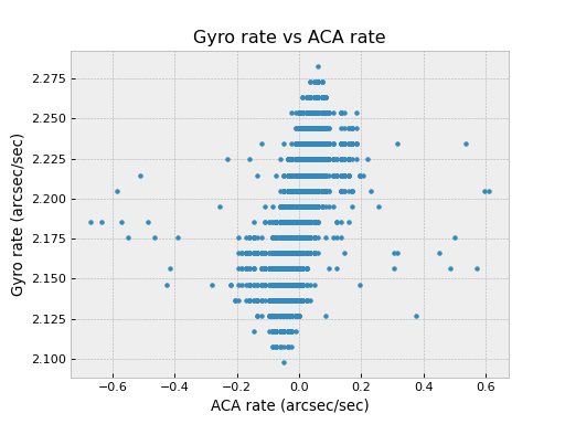
Pretend we want to look for a correlation between gyro channel 1 rate and star centroid rates in Y during an observation. We get new gyro counts every 0.25625 sec and a new centroid value every 2.05 sec.

msids = fetch.MSIDset(['aoacyan3', 'aogyrct1'], '2009:246:08:00:00', '2009:246:18:00:00')
msids.interpolate(dt=2.05)
aca_dy = msids['aoacyan3'].vals[1:] - msids['aoacyan3'].vals[:-1]
aca_dt = msids['aoacyan3'].times[1:] - msids['aoacyan3'].times[:-1]
aca_rate = aca_dy / aca_dt
gyr_dct1 = msids['aogyrct1'].vals[1:] - msids['aogyrct1'].vals[:-1]
gyr_dt = msids['aogyrct1'].times[1:] - msids['aogyrct1'].times[:-1]
gyr_rate = gyr_dct1 / gyr_dt * 0.02
clf()
plot(aca_rate, gyr_rate, '.')

Interpolation¶

The interpolate() method allows for resampling all the MSIDs in a set onto a single common time sequence. This is done by performing nearest-neighbor interpolation of all MSID values. By default the update is done in-place, but if called with copy=True then a new MSIDset() is returned and the original is not modified (see Copy versus in-place).

Times¶

The time sequence steps uniformly by dt seconds starting at the start time and ending at the stop time. If not provided the times default to the start and stop times for the MSID set.

If times is provided then this gets used instead of the default linear progression from start and dt.

For each MSID in the set the times attribute is set to the common time sequence. In addition a new attribute times0 is defined that stores the nearest neighbor interpolated time, providing the original timestamps of each new interpolated value for that MSID.

Filtering and bad values¶

A key issue in interpolation is the handling of bad (missing) telemetry values. There are two parameters that control the behavior, filter_bad and bad_union.

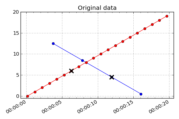
The plots and discussion below illustrate the effect of filter_bad and bad_union for a synthetic dataset consisting of two MSIDs which are sampled at 1.025 seconds (red) and 4.1 seconds (blue). The red values are increasing linearly while the blue ones are decreasing linearly. Each MSID has a single bad point which is marked with a black cross. The first plot below is the input un-interpolated data:

If filter_bad is True (which is the default) then bad values are filtered from the interpolated MSID set. There are two strategies for doing this:

bad_union = False

Remove the bad values in each MSID prior to interpolating the set to a common time series. Since each MSID has bad data filtered individually before interpolation, the subsequent nearest neighbor interpolation only finds “good” data and there are no gaps in the output. This strategy is done when bad_union = False, which is the default setting. The results are shown below: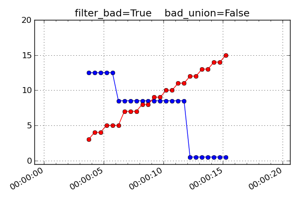
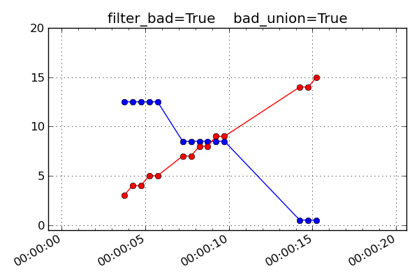
bad_union = True

Remove the bad values after interpolating the set to a common time series. This marks every MSID in the set as bad at the interpolated time if any of them are bad at that time. This stricter version is required when it is important that the MSIDs be truly correlated in time. For instance this is needed for attitude quaternions since all four values must be from the exact same telemetry sample. If you are not sure, this is the safer option because gaps in the input data are reflected as gaps in the output.

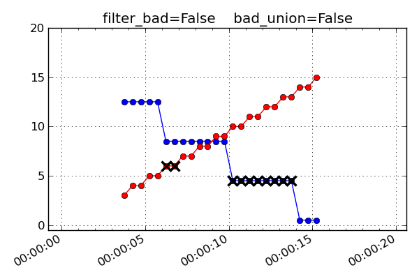
If filter_bad is False then bad values and the associated bads attribute are left in the MSID objects of the interpolated MSIDset(). The behaviors are:

bad_union = False

Bad values represent the bad status of each MSID individually at the interpolated time stamps.
bad_union = True

Bad values represent the union of bad status for all the MSIDs at the interpolated time stamps. Notice how the filter_bad = True and bad_union = True case above is exactly like this one but with the crossed-out points removed.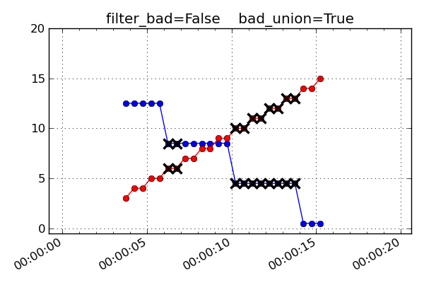

Unit systems¶

Within fetch it is possible to select a different system of physical units for the retrieved telemetry. Internally the engineering archive stores values in the FITS format standard units as used by the CXC archive. This is essentially the MKS system and features all temperatures in Kelvins (not the most convenient).

In addition to the CXC unit system one can select “science” units or “engineering” units:

System	Description
cxc	FITS standard units used in CXC archive files (basically MKS)
sci	Same as “cxc” but with temperatures in degC instead of Kelvins
eng	OCC engineering units (TDB P009, e.g. degF, ft-lb-sec, PSI)

The simplest way to select a different unit system is to alter the canonical command for importing the fetch module. To always use OCC engineering units use the following command:

from cheta import fetch_eng as fetch

This uses a special Python syntax to import the fetch_eng module but then refer to it as fetch. In this way there is no need to change existing codes (except one line) or habits. To always use “science” units use the command:

from cheta import fetch_sci as fetch

Mixing units¶

Beginning with version 0.18 of the engineering archive it is possible to reliably use the import mechanism to select different unit systems within the same script or Python process.

Example:

import cheta.fetch as fetch_cxc  # CXC units
import cheta.fetch_eng as fetch_eng
import cheta.fetch_sci as fetch_sci

t1 = fetch_cxc.MSID('tephin', '2010:001', '2010:002')
print(t1.unit  # prints "K")

t2 = fetch_eng.MSID('tephin', '2010:001', '2010:002')
print(t2.unit  # prints "DEGF")

t3 = fetch_sci.MSID('tephin', '2010:001', '2010:002')
print(t3.unit  # prints "DEGC")

MSID globs¶

Each input msid for MSID() or MSIDset() is case-insensitive and can include the linux file “glob” patterns “*”, “?”, and “[<characters>]”. See the fnmatch documentation for more details.

In the case of fetching a single MSID with fetch.MSID, the pattern must match exactly one MSID. The following are valid examples of the input MSID glob and the matched MSID:

"orb*1*_x": ORBITEPHEM1_X
"*pcadmd": AOPCADMD

The real power of globbing is for MSIDset() where you can easily choose a few related MSIDs:

"orb*1*_?": ORBITEPHEM1_X, Y and Z
"orb*1*_[xyz]": ORBITEPHEM1_X, Y and Z
"aoattqt[123]": AOATTQT1, 2, and 3
"aoattqt*": AOATTQT1, 2, 3, and 4

dat = fetch.MSIDset(['orb*1*_[xyz]', 'aoattqt*'], ...)

The msid_glob() method will show you exactly what matches a given msid:

>>> fetch.msid_glob('orb*1*_?')
(['orbitephem1_x', 'orbitephem1_y', 'orbitephem1_z'],
 ['ORBITEPHEM1_X', 'ORBITEPHEM1_Y', 'ORBITEPHEM1_Z'])

>>> fetch.msid_glob('dpa_power')
(['dpa_power'], ['DP_DPA_POWER'])

If the MSID glob matches more than 10 MSIDs then an exception is raised to prevent accidentally trying to fetch too many MSIDs (e.g. if you provided “AO*” as an input). This limit can be changed by setting the MAX_GLOB_MATCHES module attribute:

fetch.MAX_GLOB_MATCHES = 20

Finally, for derived parameters the initial DP_ is optional:

"dpa_pow*": DP_DPA_POWER
"roll": DP_ROLL

State-valued MSIDs¶

MSIDs that are state-valued such as AOPCADMD or AOECLIPS have the full state code values stored in the vals attribute. The raw count values can be accessed with the raw_vals attribute:

>>> dat = fetch.Msid('aopcadmd', '2011:185', '2011:195', stat='daily')
>>> dat.vals
array(['NMAN', 'NMAN', 'STBY', 'STBY', 'STBY', 'NSUN', 'NPNT', 'NPNT',
'NPNT', 'NPNT'],
dtype='|S4')
>>> dat.raw_vals
array([2, 2, 0, 0, 0, 3, 1, 1, 1, 1], dtype=int8)

This is handy for plotting or other analysis that benefits from a numeric representation of the values. The mapping of raw values to state code is available in the state_codes attribute:

>>> dat.state_codes
[(0, 'STBY'),
 (1, 'NPNT'),
 (2, 'NMAN'),
 (3, 'NSUN'),
 (4, 'PWRF'),
 (5, 'RMAN'),
 (6, 'NULL')]

State value counts¶

For state-valued MSIDs, the 5-minute and daily statistics include attributes that provide the count of samples within the interval for each possible state. The attribute will be named n_<STATE>s, for instance n_NMANs for AOPCADMD.

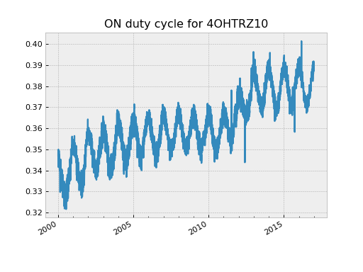
These counts are useful in at least a couple of different ways. First, one can determine the duty cycle for an ON/OFF bi-level for mission trending:

>>> dat = fetch.Msid('4ohtrz10', '2000:001', '2000:010', stat='daily')
>>> dat.n_ONs
array([3674, 3626, 3624, 3615, 3599, 3686, 3654, 3640], dtype=int32)
>>> dat.n_OFFs
array([6852, 6910, 6913, 6922, 6937, 6850, 6881, 6895], dtype=int32)
>>> dat.n_ONs * 1.0 / dat.samples
array([ 0.34975323,  0.34925005,  0.34415338,  0.34393091,  0.34307678,
        0.34159074,  0.34984814,  0.34684385,  0.34551495])

>>> dat = fetch.Msid('4ohtrz10', '2000:001', '2017:001', stat='daily')
>>> duty_cycle = dat.n_ONs * 1.0 / dat.samples
>>> plot_cxctime(dat.times, duty_cycle)
>>> plt.grid()
>>> plt.title('ON duty cycle for 4OHTRZ10')

Second, one can use the state counts to very quickly look for rare occurrences of an MSID in a particular state. As an example we can easily find every time that PCAD reported being in bright star hold (AOACASEQ == 'BRIT'). This could occur due to an autonomous safing action or as part of a realtime recovery activity. In any case searching the full-resolution telemetry is slow and memory intensive, but doing this via the daily state code counts is a snap:

>>> dat = fetch.Msid('aoacaseq', '2000:001', stat='daily')
>>> ok = dat.n_BRITs > 10  # Require at least 10 BRIT samples
>>> print([d[:8] for d in DateTime(dat.times[ok]).date])
['2000:049', '2001:111', '2001:112', '2001:265', '2002:024', '2003:200', '2004:200',
 '2004:208', '2004:213', '2004:315', '2004:316', '2008:225', '2008:226', '2008:227',
 '2008:294', '2010:151', '2011:190', '2011:192', '2011:299', '2011:300', '2012:151',
 '2014:207', '2015:007', '2015:264', '2015:265', '2016:064', '2016:234', '2016:324',
 '2016:325']

One could then drill down on these dates using 5-minute or full-resolution telemetry.

Telemetry database¶

With an MSID() object you can directly access all the information in the Chandra Telemetry Database which relates to that MSID. This is done through the Ska.tdb module. For example:

>>> dat = fetch.Msid('aopcadmd', '2011:187', '2011:190')

>>> dat.tdb  # Top level summary of TDB info for AOPCADMD
<MsidView msid="AOPCADMD" technical_name="PCAD MODE">

>>> dat.tdb.Tsc  # full state codes table
rec.array([('AOPCADMD', 1, 1, 0, 0, 'STBY'), ('AOPCADMD', 1, 7, 6, 6, 'NULL'),
           ('AOPCADMD', 1, 6, 5, 5, 'RMAN'), ('AOPCADMD', 1, 5, 4, 4, 'PWRF'),
           ('AOPCADMD', 1, 4, 3, 3, 'NSUN'), ('AOPCADMD', 1, 2, 1, 1, 'NPNT'),
           ('AOPCADMD', 1, 3, 2, 2, 'NMAN')],
          dtype=[('MSID', '|S15'), ('CALIBRATION_SET_NUM', '<i8'),
                 ('SEQUENCE_NUM', '<i8'), ('LOW_RAW_COUNT', '<i8'),
                 ('HIGH_RAW_COUNT', '<i8'), ('STATE_CODE', '|S4')])

>>> dat.tdb.Tsc['STATE_CODE']  # STATE_CODE column
rec.array(['STBY', 'NULL', 'RMAN', 'PWRF', 'NSUN', 'NPNT', 'NMAN'],
          dtype='|S4')

>>> dat.tdb.technical_name
'PCAD MODE'

>>> dat.tdb.description
'LR/15/SD/10 PCAD_MODE'

Note that the tdb attribute is equivalent to Ska.tdb.msids[MSID], so refer to the Ska.tdb documentation for further information.

MAUDE telemetry server¶

The fetch module provides the capability to choose the source of telemetry data used in queries. The historical (and current default) source of telemetry data consists of a collection of HDF5 files that are constructed and updated daily using CXC level-0 engineering telemetry decom products. This has the bulk of commonly used telemetry but typically has a latency of 2-3 days.

In order to fill this gap an interface to the MAUDE telemetry server is also available.

The key differences between the CXC and MAUDE telemetry data sources are:

CXC includes pseudo-MSIDs such as ephemeris data, ACIS and HRC housekeeping, and derived parameters like the pitch and off-nominal roll angle.
CXC has a latency of 2-3 days vs. hours for MAUDE back-orbit telemetry.
During a realtime support MAUDE provides real-time telemetry.
CXC has about 6800 MSIDs while MAUDE has around 11350. At least some of the MSIDs that are only in MAUDE are somewhat obscure ones like ACIMG1D1 (PEA1 PIXEL D1 DATA IMAGE 1) which the CXC decoms into higher-level products.
CXC is optimized for large bulk queries using direct disk access. It is limited only by system memory (gigabytes) and always returns all available data points.
MAUDE is optimized for smaller, more frequent queries and uses a secure web server to provide data. It has limits on both the number of returned data values (around 100k) and the total number of bytes in the data (around 1.6 Mb).
By default MAUDE will sub-sample the data as necessary to fit in the data limits (see below for example of disabling this feature).

Basic usage¶

Once you have followed the steps to Setup for MAUDE authentication, you can access the MAUDE data.

The source of data for fetch queries is controlled by the module-level fetch.data_source configuration object. You can first view the current data source with:

>>> fetch.data_source.sources()
('cxc',)

This shows that the current source of data is the CXC files. You can change to MAUDE as follows:

>>> fetch.data_source.set('maude')
>>> fetch.data_source.sources()
('maude',)

Now if you execute a query MAUDE will be used. There is not any obvious difference from the user perspective and the returned Msid object looks and behaves exactly as if you had queried from the CXC data:

>>> dat = fetch.Msid('tephin', '2015:001', '2015:002')

The most direct way to be sure of the actual data source is to look at the data_source attribute:

>>> dat.data_source
{'maude': {'flags': {'subset': False, 'tolerance': False},
           'start': '2015:001:12:00:15.037',
           'stop': '2015:002:11:59:37.452'}}

This shows the start and stop time for data values that were returned by the MAUDE server. In addition two status flags are returned.

Data subsets

For the purposes here, the important flag is subset. As mentioned above, the MAUDE server will not return more than around 100k data values in a single query. When a query would return more than this number of values then the server automatically subsamples the data to return no more than 100k points. This is done in a clever way such that it reproduces what a plot of the fully-sampled dataset would look like at screen resolution. Nevertheless one should pay attention to the subset flag, particularly in cases where subsampling could affect analysis results. One example is examinine attitude quaternions (AOATTQT{1,2,3,4}) where the four values must be taken from the exact same readout frame.

In order to force the MAUDE server to return full resolution data, the MAUDE data source needs to be configured with the allow_subset=False flag. This will prevent sub-sampling by doing multiple small queries. This has an overhead penalty because it may require multiple server requests to piece together the full query. For example:

>>> import maude
>>> maude.set_logger_level(10)  # Show debugging information from maude
>>> fetch.data_source.set('maude allow_subset=False')
>>> dat = fetch.Msid('aoattqt1', '2016:001', '2016:003')
get_msids: Using .netrc with user=taldcroft
get_msids_in_chunks: Chunked reading: max samples / major_frame = 32, chunk dt = 82000.0 secs
get_msids: Getting URL http://t...cfa.harvard.edu/...&ts=2016001120000000&tp=2016002040000000
get_msids: Getting URL http://t...cfa.harvard.edu/...&ts=2016002040000000&tp=2016002200000000
get_msids: Getting URL http://t...cfa.harvard.edu/...&ts=2016002200000000&tp=2016003120000000
>>> len(dat.vals)
168586  # MORE than 100000!

When allow_subset=False then a fetch query is not allowed to span more than 7 days in order to prevent swamping the MAUDE server.

Multiple data sources

A common use case (indeed a key driver for accessing MAUDE through the Ska interface) is to fetch data using both the CXC and MAUDE data, taking CXC data where possible and then filling in the last couple of days using MAUDE with full-resolution data (no subsetting). This is done by specifying the data source as both cxc and maude allow_subset=False, as shown in the following example:

>>> fetch.data_source.set('cxc', 'maude allow_subset=False')

Now assume the current date is 2016:152:01:00:00 and we want all available data since 2016:100

>>> dat = fetch.Msid('tephin', '2016:100')
>>> dat.data_source
{'cxc': {'start': '2016:100:12:00:11.268',
         'stop': '2016:150:19:38:40.317'},
 'maude': {'flags': {'subset': False, 'tolerance': False},
           'start': '2016:150:19:38:56.130',
           'stop': '2016:151:20:40:37.392'}}

This shows that data have been fetched from both data sources and stitched together seamlessly.

Context manager¶

The fetch.data_source object can also be used as a context manager to temporarily change the data source within an enclosed code block. This is useful because it restores the original data source even if there is an exception within the code block. For instance:

>>> fetch.data_source.sources()
('cxc',)
>>> with fetch.data_source('maude'):
...     dat = fetch.Msid('tephin', '2016:001', '2016:002')
...     print(fetch.data_source.sources())
...
('maude',)
>>> fetch.data_source.sources()
('cxc',)

Data source differences¶

There are different MSIDs available in the different data sources (but mostly they overlap). To directly understand this you can access the MSID lists as follows. The get_msids() method of data_source returns a Python set of MSIDs:

>>> cxc_msids = fetch.data_source.get_msids('cxc')
>>> maude_msids = fetch.data_source.get_msids('maude')
>>> sorted(cxc_msids - maude_msids)  # In CXC but not MAUDE
['3W00FILL',
 '3W05FILL',
 '3W22FILL',
 ...
 'TMP_FEP1_MONG',
 'TMP_FEP1_PCB',
 'TMP_FEP1_RAM']

>>> len(cxc_msids - maude_msids)
552
>>> len(maude_msids - cxc_msids)
5107

If you do a mixed-source query (CXC and MAUDE) for an MSID that is available in only one of the sources, then just the one source will be used. For instance:

>>> dat = fetch.Msid('pitch', '2016:145')  # from 2016:145 to present
>>> dat.data_source
{'cxc': {'start': '2016:145:12:00:00.241',
         'stop': '2016:150:18:37:01.841'}}

Setup for MAUDE authentication¶

In order to use MAUDE as the data source you must have authentication credentials (username and password) to access OCCweb. One can provide those credentials manually to the get_msids() function call, but this gets tiresome.

The preferred method to use this from a secure machine is to edit the file .netrc in your home directory and put in your OCCweb credentials.

IMPORTANT: make sure the file is readable only by you!

chmod og-rwx ~/.netrc

Once you have done that, add these three lines. If there are already other machines defined you need a blank line between the machine configs.

machine  occweb
login    your-occweb-username
password your-occweb-password

Pushing it to the limit¶

The engineering telemetry archive is designed to help answer questions that require big datasets. Let’s explore what is possible. First quit from your current ipython session with exit(). Then start a window that will let you watch memory usage:

xterm -geometry 80x15 -e 'top -u <username>' &

This brings up a text-based process monitor. Focus on that window and hit “M” to tell it to order by memory usage. Now go back to your main window and get all the TEIO data for the mission:

ipython --matplotlib
import cheta.fetch as fetch
import matplotlib.pyplot as plt
from Ska.Matplotlib import plot_cxctime
time teio = fetch.MSID('teio', '2000:001', '2010:001', filter_bad=True)
Out[]: CPU times: user 2.08 s, sys: 0.49 s, total: 2.57 s
       Wall time: 2.85 s

Now look at the memory usage and see that around a 1 Gb is being used:

len(teio.vals) / 1e6
plt.clf()
plot_cxctime(teio.times, teio.vals, '.', markersize=0.5)

Making a plot with 13 million points takes 5 to 10 seconds and some memory. See what happens to memory when you clear the plot:

plt.clf()

Now let’s get serious and fetch all the AORATE3 values (1 per second) for the mission after deleting the TEIO data:

del teio
%time aorate3 = fetch.MSID('aorate3', '2000:001', '2010:001', filter_bad=True)
Out[]: CPU times: user 38.83 s, sys: 7.43 s, total: 46.26 s
       Wall time: 60.10 s

We just fetched 300 million floats and now top should be showing some respectable memory usage:

Cpu(s):  0.0%us,  0.1%sy,  0.0%ni, 99.7%id,  0.2%wa,  0.1%hi,  0.0%si,  0.0%st

  PID USER      PR  NI  VIRT  RES  SHR S %CPU %MEM    TIME+  COMMAND
14243 aca       15   0 6866m 6.4g  11m S  0.0 40.9   3:08.70 ipython

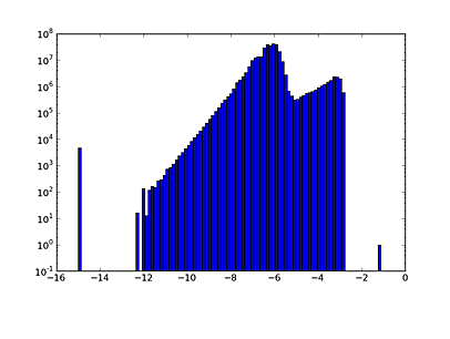
If you try to make a simple scatter plot with 300 million points you will make the machine very unhappy. But we can do computations or make a histogram of the distribution:

plt.clf()
plt.hist(np.log10(abs(aorate3.vals)+1e-15), log=True, bins=100)

Rules of thumb:

1 million is fast for plotting and analysis.
10 million is fast for analysis but on the edge for plotting:
- Plotting lines or symbols (the '-' or '.' markers) may fail with the dreaded Agg rendering complexity exceeded. Once this happens you frequently need to restart IPython entirely to make more plots.
- Plotting with the ',' marker is typically OK as this just makes a single pixel dot instead of a plot glyph.
300 million is OK for analysis, expect 30-60 seconds for any operation. Plots can only be done using density image maps binning in 2-d.
Look before you leap, do smaller fetches first and check sizes as shown below.
5-minute stats are ~10 million so you are always OK.

Estimating fetch size¶

You can do a better than the above rules of thumb using the get_fetch_size() function in the cheta.utils module to estimate the size of a fetch request prior to making the call. This is especially useful for applications that want to avoid unreasonably large data requests.

As an example, compute the estimated size in Megabytes for fetching full-resolution data for TEPHIN and AOPCADMD for a period of 3 years, both of which are then interpolated at a time sampling of 32.8 seconds:

>>> from cheta.utils import get_fetch_size
>>> get_fetch_size(['TEPHIN', 'AOPCADMD'], '2011:001', '2014:001', interpolate_dt=32.8)
(1248.19, 75.06)

This returns two numbers: the first is the memory (megabytes) for the internal fetch operation to get the telemetry data, and the second is the memory for the interpolated output. This estimate is made by fetching a 3-day sample of data starting at 2010:001 and extrapolating. Therefore the size estimates are reflective of normal operations.

Fetching the easy way¶

The high-level function get_telem() is available to simplify use of the Ska engineering archive. It provides a way to combine many of the common processing steps associated with fetching and using telemetry data into a single function call. This includes:

Fetch a set of MSIDs over a time range, specifying the sampling as either full-resolution, 5-minute, or daily data.
Filter out bad or missing data.
Interpolate (resample) all MSID values to a common uniformly-spaced time sequence.
Remove or select time intervals corresponding to specified Kadi event types.
Change the time format from CXC seconds (seconds since 1998.0) to something more convenient like GRETA time.
Write the MSID telemetry data to a zip file.

Aside from the first two steps (fetching data and filtering bad data), all the steps are optional.

The get_telem() function has a lot of parameters in order to be flexible, but we’ll break them down into manageable groups.

Desired telemetry

The first set are the key inputs relating to the actual telemetry:

Argument	Description
msids	MSID(s) to fetch (string or list of strings)
start	Start time for data fetch (default=<stop> - 30 days)
stop	Stop time for data fetch (default=NOW)
sampling	Data sampling (full \| 5min \| daily) (default=full)’)
unit_system	Unit system for data (eng \| sci \| cxc) (default=eng)

The first argument msids is the only one that always has to be provided. It should be either a single string like 'COBSRQID' or a list of strings like ['TEPHIN', 'TCYLAFT6', 'TEIO']. Note that the MSID is case-insensitive so 'tephin' is fine.

The start and stop arguments are typically a string like '2012:001:02:03:04' (ISO time) or '2012001.020304' (GRETA time). If not provided then the last 30 days of telemetry will be fetched.

The sampling argument will choose between either full-resolution telemetry or the 5-minute or daily summary statistic values.

The unit_system argument selects the output unit system. The choices are engineering units (i.e. what is in the TDB and GRETA), science units (mostly just temperatures in C instead of F), or CXC units (whatever is in CXC decom, which e.g. has temperatures in K).

Example:

% ska
% ipython --pylab
>>> from cheta.fetch import get_telem
>>> dat = get_telem(['tephin', 'tcylaft6'], '2010:001', '2010:030', sampling='5min')
>>> clf()
>>> dat['tephin'].plot(label='TEPHIN', color='r')
>>> dat['tcylaft6'].plot(label='TCYLAFT6', color='b')
>>> legend()

The output of get_telem() is an MSIDset() object which is described in the MSID sets section.

Interpolation

Argument	Description
interpolate_dt	Interpolate to uniform time steps (secs, default=None)

In general different MSIDs will come down in telemetry with different sampling and time stamps. Interpolation allows you to put all the MSIDs onto a common time sequence so you can compare them, plot one against the other, and so forth. You can see the Interpolation section for the gory details, but if you need to have your MSIDs on a common time sequence then set interpolate_dt to the desired time step in seconds. When interpolating get_telem() uses filter_bad=True and union_bad=True (as described in Interpolation).

Intervals

Argument	Description
remove_events	Remove kadi events expression (default=None)
select_events	Select kadi events expression (default=None)

These arguments allow you to select or remove intervals in the data using the Kadi event definitions. For instance we can select times of stable NPM dwells during radiation zones:

>>> dat = get_telem(['aoatter1', 'aoatter2', 'aoatter3'],
                    start='2014:001', stop='2014:010', interpolate_dt=32.8,
                    select_events='dwells & rad_zones')

The order of processing is to first remove event intervals, then select event intervals.

The expression for remove_events or select_events can be any logical expression involving Kadi query names (see the event definitions table). The following string would be valid: 'dsn_comms | (dwells[pad=-300] & ~eclipses)', and for select_events this would imply selecting telemetry which is either during a DSN pass or (within a NPM dwell and not during an eclipse). The [pad=-300] qualifier means that a buffer of 300 seconds is applied on each edge to provide padding from the maneuver. A positive padding expands the event intervals while negative contracts the intervals.

Output

Argument	Description
time_format	Output time format (secs\|date\|greta\|jd\|…, default=secs)
outfile	Output file name (default=None)

By default the times attribute for each MSID is provided in seconds since 1998.0 (CXC seconds). The time_format argument allows selecting any time format supported by Chandra.Time.

If the outfile is set to a valid file name then the MSID set will be written out as a compressed zip archive. This archive will contain a CSV file corresponding to each MSID in the set. See the section on Exporting to CSV for additional information and an example of the output format.

Process control

Argument	Description
quiet	Suppress run-time logging output (default=False)
max_fetch_Mb	Max allowed memory (Mb) for fetching (default=1000)
max_output_Mb	Max allowed memory (Mb) for output (default=100)

Normally get_telem() outputs a few lines of progress information as it is processing the request. To disable this logging set quiet=True.

The next two arguments are in place to prevent accidentally doing a huge query that will consume all available memory or generate a large file that will be slow to read. For instance getting all the gyro count data for the mission will take more than 70 Gb of memory.

The max_fetch_Mb argument specifies how much memory the fetched MSIDset() can take. This has a default of 1000 Mb = 1 Gb.

The max_output_Mb only applies if you have also specified an outfile to write. This checks the size of the actual output MSIDset(), which may be smaller than the fetch object if data sampling has been reduced via the interpolate_dt argument. This has a default of 100 Mb.

Both of the defaults here are relatively conservative, and with experience you can set larger values.

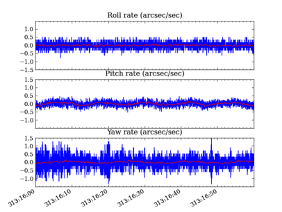
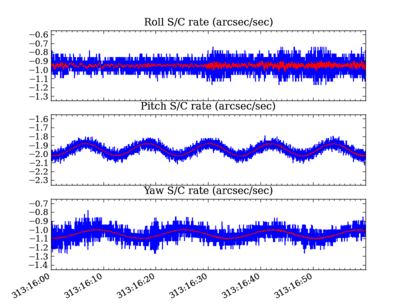
Putting it all together¶

As a final example here is a real-world problem of wanting to compare OBC rates to those derived on the ground using raw gyro data.

import cheta.fetch as fetch
from Ska.Matplotlib import plot_cxctime
import Ska.Numpy

tstart = '2009:313:16:00:00'
tstop = '2009:313:17:00:00'

# Get OBC rates and gyro counts
obc = fetch.MSIDset(['aorate1', 'aorate2', 'aorate3'], tstart, tstop, filter_bad=True)
gyr = fetch.MSIDset(['aogyrct1', 'aogyrct2', 'aogyrct3', 'aogyrct4'], tstart, tstop, filter_bad=True)

# Transform delta gyro counts (4 channels) to a body rate (3 axes)
cts2rate = array([[-0.5       ,  0.5       ,  0.5       , -0.5       ],
                  [-0.25623091,  0.60975037, -0.25623091,  0.60975037],
                  [-0.55615682, -0.05620959, -0.55615682, -0.05620959]])

# Calculate raw spacecraft rate directly from gyro data
cts = np.array([gyr['aogyrct1'].vals,
                gyr['aogyrct2'].vals,
                gyr['aogyrct3'].vals,
                gyr['aogyrct4'].vals])
raw_times = (gyr['aogyrct1'].times[1:] + gyr['aogyrct1'].times[:-1]) / 2
delta_times = gyr['aogyrct1'].times[1:] - gyr['aogyrct1'].times[:-1]
delta_cts = cts[:, 1:] - cts[:, :-1]
raw_rates = np.dot(cts2rate, delta_cts) * 0.02 / delta_times

# Plot the OBC rates
figure(1, figsize=(8,6))
clf()
for frame, msid, label in ((1, 'aorate1', 'roll'),
                           (2, 'aorate2', 'pitch'),
                           (3, 'aorate3', 'yaw')):
    subplot(3, 1, frame)
    obc_rates = obc[msid].vals * 206254.
    plot_cxctime(obc[msid].times, obc_rates, '-')
    plot_cxctime(obc[msid].times, Ska.Numpy.smooth(obc_rates, window_len=20), '-r')
    ylim(average(obc_rates) + array([-1.5, 1.5]))
    title(label.capitalize() + ' rate (arcsec/sec)')

subplots_adjust(bottom=0.12, top=0.90)
# savefig('obc_rates.png')

# Plot the S/C rates from raw gyro data
figure(2, figsize=(8,6))
clf()
for axis, label in ((0, 'roll'),
                    (1, 'pitch'),
                    (2, 'yaw')):
    subplot(3, 1, 1+axis)
    raw_rate = raw_rates[axis, :]
    plot_cxctime(raw_times, raw_rate, '-')
    plot_cxctime(raw_times, Ska.Numpy.smooth(raw_rate, window_len=20), '-r')
    ylim(np.mean(raw_rate) + np.array([-0.4, 0.4]))
    title(label.capitalize() + ' S/C rate (arcsec/sec)')

subplots_adjust(bottom=0.12, top=0.90)
# savefig('gyro_sc_rates.png')

Remote data access¶

The telemetry archive can be accessed remotely if ssh access to chimchim is available. The user will be queried for ssh credentials and fetch will connect with a controller running on chimchim to retrieve the data. Besides the initial query for credentials (and slower speeds when fetching data over the network), the use of fetch is essentially the same whether the archive is local or remote.

In order to use this option, the user must have a special key file ska_remote_access.json placed at the root of the local Python installation folder. This is placed in the directory shown with import sys; print(sys.prefix).

To get a copy of this file contact Mark Baski or Tom Aldcroft, or look in the DAWG_TIPS_AND_TRICKS topic in the SpecialProjects Web on the TWiki.

Remote access is controlled as follows:

The environment variable SKA_ACCESS_REMOTELY can be set to “False” or “True” to force either disabling or enabling remote access, respectively.
If SKA_ACCESS_REMOTELY is not defined on a linux or Mac system, remote access is always disabled.
If SKA_ACCESS_REMOTELY is not defined on a Windows system, remote access is enabled unless the system finds a local engineering data archive. It looks for data in either $SKA/data/eng_archive or $ENG_ARCHIVE, where those refer to user-defined environment variables.
If remote access is disabled and there is no local engineering data archive, then a warning is issued. In this case you can still use MAUDE for data access with fetch.data_source.set('maude').

Scripts using remote access¶

If you are using remote data access from within a script, you should write the script using calls to functions instead of having everything at the main level. For example:

from cheta import fetch

def main():
    # For remote access this will interactively prompt the user for an
    # IP address, user name and password (for only the first fetch).
    dat = fetch.Msid('tephin', '2020:001', '2020:002')

    # Now do something with dat
    print(dat)

if __name__ == '__main__':
    main()

The reason for this is that the code which accesses the remote server may end up importing the main script many times, so if you have non-trivial code at the top level this causes problems. For example:

# DO NOT DO THIS
from cheta import fetch

# This line gets run multiple times in succession via multiprocessing: FAIL
dat = fetch.Msid('tephin', '2020:001', '2020:002')

These problems are known to happen on Windows, but following this best practice should be done for all remote-access scripts.

Local cheta archive¶

Instructions for creating, using, and maintaining a local cheta archive (on your laptop for instance) are found at the Tutorial for installing and maintaining a cheta telemetry archive.

Navigation

Fetch Tutorial¶

Getting started¶

Date and time formats¶

Exporting to CSV¶

Plotting time data¶

Interactive plotting¶

Data filtering¶

Event interval filtering¶

Using Kadi¶

Using logical intervals¶

Fetching only small intervals¶

Bad data¶

Really bad data¶

Filtering out arbitrary time intervals¶

Copy versus in-place¶

Five minute and daily stats¶

MSID sets¶

Interpolation¶

Times¶

Filtering and bad values¶

Unit systems¶

Mixing units¶

MSID globs¶

State-valued MSIDs¶

State value counts¶

Telemetry database¶

MAUDE telemetry server¶

Basic usage¶

Context manager¶

Data source differences¶

Setup for MAUDE authentication¶

Pushing it to the limit¶

Estimating fetch size¶

Fetching the easy way¶

Putting it all together¶

Remote data access¶

Scripts using remote access¶

Local cheta archive¶